How to create dependent drop-down list in MS-Excel?

In this blog, I will explain how to create a dependent drop-down list in Microsoft-Excel. A dependent drop-down list is a list in which one particular field, depends on the other.

The advantages of dropdowns include saving screen space, and also preventing users from entering erroneous data since they have only predefined values to choose from. It is quick and more accurate. Through an example of the table given below, we will learn what is a dependent drop-down list and how to create one.

In the table below, a dependent drop-down list will be formed in columns B and C, so that when a country is selected, the cities for that particular country are shown. These lists can be made for many purposes and not just the one mentioned here like countries and their cities. A snapshot of the excel which we will be using as an example is given below.

You can also learn this by watching our YouTube video.

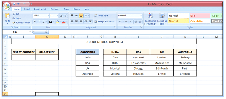
You can follow these steps to create a drop-down list:

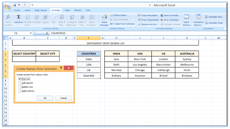
• First, select the row naming the countries i.e. F4-F7 in this case. Now, click on 'Formula' ribbon and there select 'Create from selection'; then select 'Top row' and click on OK.

Go to Formula -> Create from Selection -> Select Top Row.

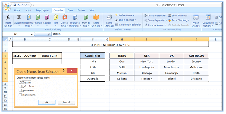
• In the same way, select the next table showing the names of cities of each country, click on the 'Formula' ribbon; select 'Create from selection'; click on 'Top row' and then OK. 

Go to Formula -> Create from Selection -> Select Top Row.

Now the next thing we want is that when we mention the name of a country in B4, we see the names of cities (mentioned in the other table) of that country in C4. So for that, we have to create a dropdown.

To create this dropdown, click on the ‘Data’ ribbon. Select ‘Data validation’. A table will appear on the screen namely 'Data Validation'. There, in 'Allow' - select 'List'

Go to Data -> Data Validation -> Allow-select List

Next, in the same table, go to the 'Source' option and then select the row mentioning countries i.e. from F3 to F7 and finally click on OK.

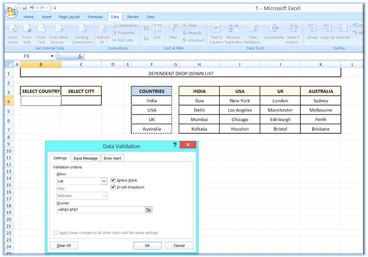
You will see that a dropdown icon has appeared near the selected cell i.e. B4 in this case.

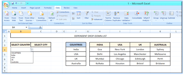
Next, we want to see the names of the cities in C4. To accomplish that, we have to start with the same process, click on 'Data' ribbon. Go to 'Data validation'. In the table that appears, select 'List' in the allow option.

The only difference here is that in the source option, you have to apply a formula which is as follows: =INDIRECT(select the source i.e. B4 cell in this case) and click on OK.

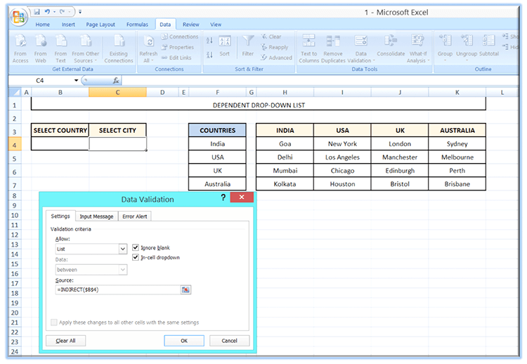
After this step, you will a dropdown icon near C4 too, when you select the country in B4. Here you can choose the city.

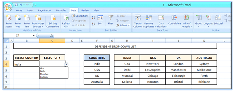
You can see now that creating a dependent drop-down list may have seemed difficult at first sight, but it is quite facile and simple. We hope that this write-up has made the process simpler for you.

Please leave your comments below and don't forget to subscribe to our website for more such solutions.